20: Correlation

Setting

We will once again visualize the act of ordering food at In-n-Out.

• $X$: number of fries orders
• $Y$: number of beef patties ordered

joint PMF

Covariance

We define the covariance of random variables as

$$\text{Cov}(X,Y)=\text{E}[XY]-\text{E}[X]\text{E}[Y]$$

Correlation

Correlation

Just like how the $z$-score is a standardized and unitless measure, the correlation was designed to be standardized and unitless (i.e. units cancel out).

$$r=\text{Corr}(X,Y)={\displaystyle \frac{\text{Cov}(X,Y)}{\sqrt{\text{Var}(X)\cdot \text{Var}(Y)}}}$$

• If $\text{Var}(X)=0$, the data $X$ are constant, and simply return $r=0$
• If $\text{Var}(Y)=0$, the data $Y$ are constant, and simply return $r=0$

• Compute the correlation in the In-n-Out setting

Interpretation of Correlation

Ranges

Ranges

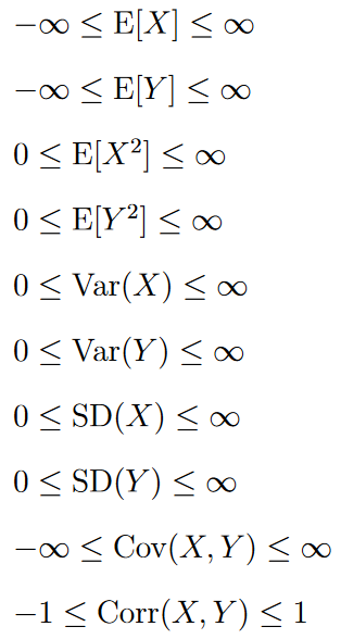
Aside: the infinity-sized expected values might happen in continuous distributions.

Interpretation of Correlation

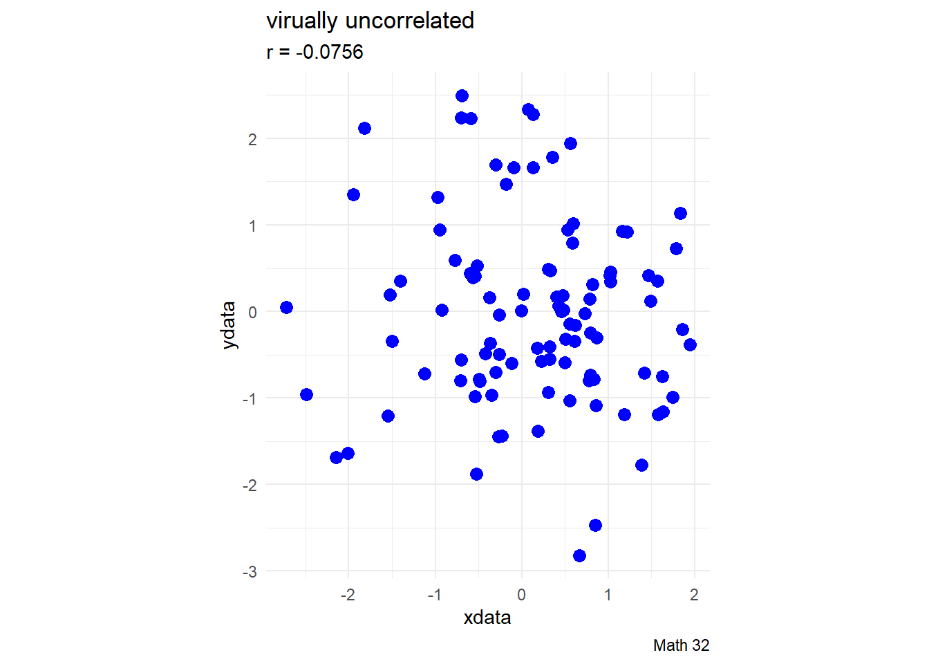
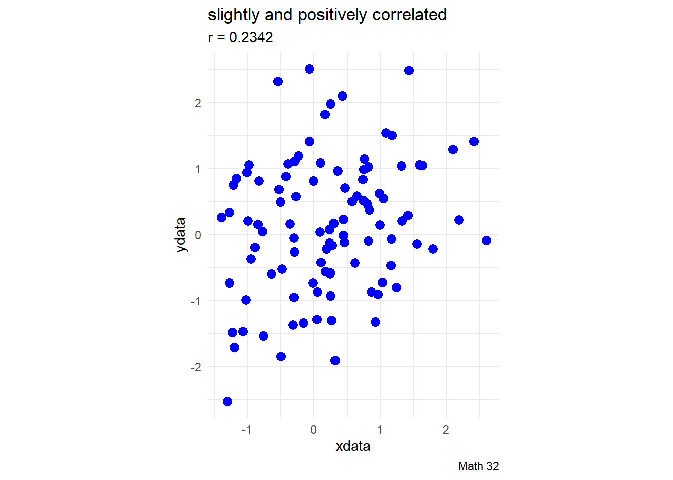
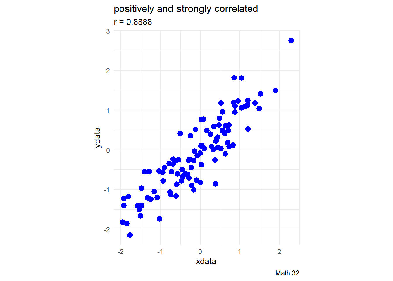
Early development of the concept of correlation was done by Karl Pearson. Pearson suggested the following interpretations of the correlation (but there is no strict rule for this):

• $|r|<0.4$: virtually uncorrelated
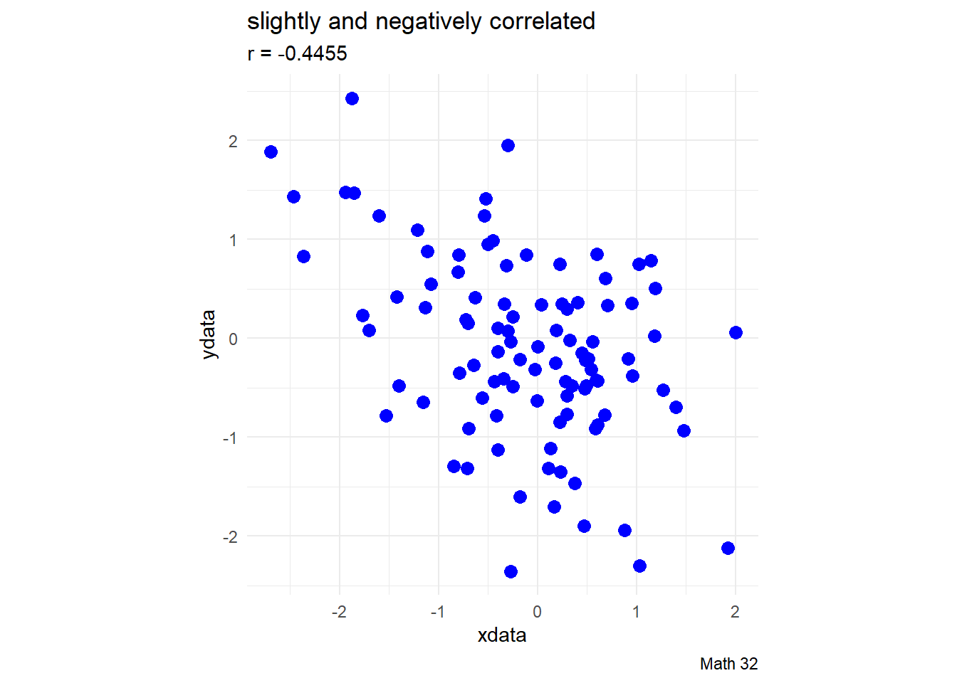
• $0.4\le |r|<0.7$: slightly correlated
• $0.7\le |r|\le 1.0$: strongly correlated

Examples of Correlation

R

correlatedValues = function(x, r = 0.9){
  r2 = r**2
  ve = 1-r2
  SD = sqrt(ve)
  e  = rnorm(length(x), mean=0, sd=SD)
  y  = r*x + e
  return(y)
}

x1 = rnorm(100, mean = 0, sd = 1)
y1 = correlatedValues(x1, r = -0.9)
x2 = rnorm(100, mean = 0, sd = 1)
y2 = correlatedValues(x2, r = -0.4)
x3 = rnorm(100, mean = 0, sd = 1)
y3 = correlatedValues(x3, r = 0.0)
x4 = rnorm(100, mean = 0, sd = 1)
y4 = correlatedValues(x4, r = 0.4)
x5 = rnorm(100, mean = 0, sd = 1)
y5 = correlatedValues(x5, r = 0.9)

df1 <- data.frame(x1, y1, "group 1")
df2 <- data.frame(x2, y2, "group 2")
df3 <- data.frame(x3, y3, "group 3")
df4 <- data.frame(x4, y4, "group 4")
df5 <- data.frame(x5, y5, "group 5")
names(df1) <- c("xdata", "ydata", "group")
names(df2) <- c("xdata", "ydata", "group")
names(df3) <- c("xdata", "ydata", "group")
names(df4) <- c("xdata", "ydata", "group")
names(df5) <- c("xdata", "ydata", "group")
main_df <- rbind(df1, df2, df3, df4, df5)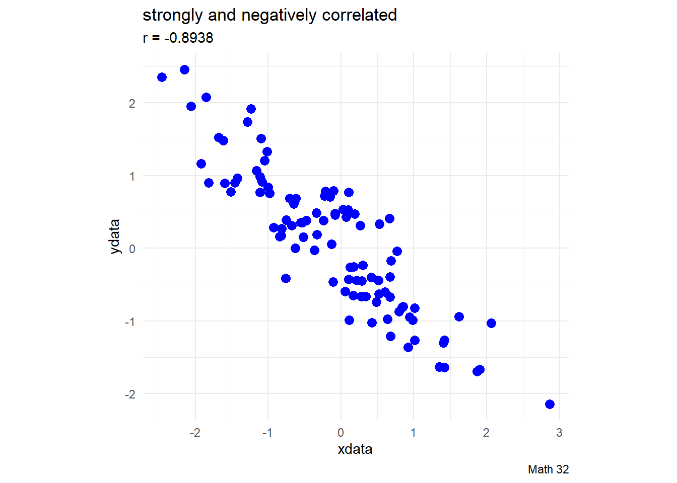

1

2

3

4

5

Continuous Joint Probability Distribution Functions

We will once again visualize the act of ordering food at In-n-Out.

• $X$: number of fries orders
• $Y$: number of beef patties ordered

with joint PDF

$$f(x,y)=\frac{1}{30}(x+y)e^{-x}{e}^{-y/5}$$

• Compute the correlation in the In-n-Out setting

In-n-Out

Looking Ahead

• due Fri., Mar. 17:

  • WHW8
  • LHW7

• Exam 2 will be on Mon., Apr. 10

• no lecture on Mar. 24, Apr. 3

tweet source