24: Estimators

Today: Estimators

Goal: Explore generalization from samples to populations

Objectives: Show the biased or unbiased estimation via

• sample mean $\overline{x}$
• sample variance $s^2$
• sample standard deviation $s$

Demographics Example

From our Demographics Survey data of Math 32 students, suppose that the following is a sample of observations of heights (in inches):

$$\{x_{11}=72,x_{12}=61,x_{13}=60,x_{14}=75,x_{15}=69\}$$

• then $t_1=67.4$ inches is the sample mean.

Suppose that the following is another sample of heights:

$$\{x_{21}=66,x_{22}=78,x_{23}=78,x_{24}=77,x_{25}=64\}$$

• then $t_2=72.6$ inches is the sample mean.

Suppose that the following is another sample of heights:

$$\{x_{31}=61,x_{32}=59,x_{33}=70,x_{34}=61,x_{35}=65\}$$

• then $t_3=63.2$ inches is the sample mean.

Sampling Itself is Probabilistic

Observe: the sample mean (usually) changes upon a new set of observations

• Can we calculate the average height of UC Merced students?
• How can we calculate the average height of UC Merced students?

Thought: what if we take a mean of the sample means?

Estimators

Estimators

Let $T$ be a random variable and $f$ be some calculation $$T=f(x_1,x_2,x_3,...)$$

If we are trying to estimate a population parameter $\theta$, we say that $T$ is an unbiased estimator of $\theta$ if $$\text{E}[T]=\theta$$

Today, we will look at situations where $f$ is calculating the

• mean
• variance
• standard deviation

Mean

Setup

We will run simulations with $X\sim U(0,1)$ because we know what the answers should be. The population mean is

$$\mu ={\displaystyle \frac{a+b}{2}={\displaystyle \frac{1}{2}}}$$

Code

N <- 1337 # number of iterations
n <- 25   # sample size

# pre-allocate vector of space for observations
obs <- rep(NA, N)

# run simulation
for(i in 1:N){
  these_numbers <- runif(n, 0, 1) # sample n numbers from U(0,1)
  obs[i] <- mean(these_numbers) #record average
}

# mean of observations
mean_of_obs <- mean(obs)

# make data frame
df <- data.frame(obs)

# visualization
df |>
  ggplot(aes(x = obs)) +
  geom_density(color = "black", size = 2) +
  geom_vline(xintercept = 1/2, color = "red", size = 3) +
  labs(title = "Simulation Sample Mean",
       subtitle = paste("black: sample distribution\nred: true population mean\nmean of sample means: ", round(mean_of_obs, 4)),
       caption = "Math 32") +
  theme_minimal()

Simulation

Warning: Using `size` aesthetic for lines was deprecated in ggplot2 3.4.0.
ℹ Please use `linewidth` instead.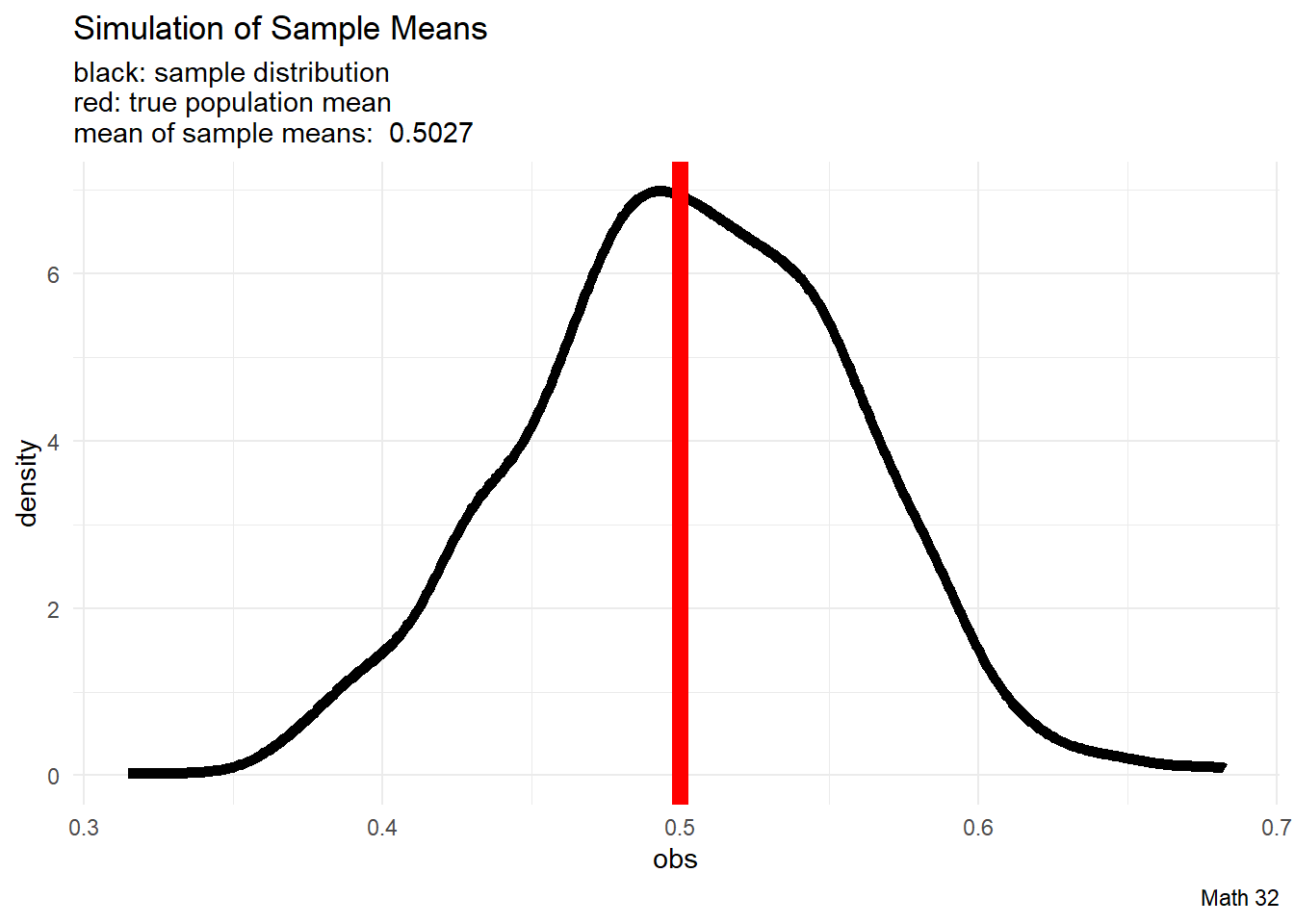

Loosely speaking, since the sampling distribution “lines up” with the population mean, we say that the sample median is an unbiased estimator of the population mean.

Proof

$$\begin{array}{rcl}\text{E}[{\overline{X}}_n]& =& \text{E}\left({\displaystyle \frac{X_1+X_2+...+X_n}{n}}\right)\\ & =& {\displaystyle \frac{1}{n}\text{E}(X_1+X_2+...+X_n)}\\ & =& {\displaystyle \frac{1}{n}(\text{E}[X_1]+\text{E}[X_2]+...+\text{E}[X_n])}\\ & =& {\displaystyle \frac{1}{n}(\mu +\mu +...+\mu )}\\ & =& {\displaystyle \frac{1}{n}\left(n\mu \right)}\end{array}$$

Therefore $\text{E}[{\overline{X}}_n]=\mu$

Population Variance

Setup

We will run simulations with $X\sim U(0,1)$ because we know what the answers should be. The population variance is

$${\sigma }^2={\displaystyle \frac{(b-a{)}^2}{12}={\displaystyle \frac{1}{12}}}$$

We will explore what happens if we apply the population variance formula

$${\sigma }^2=\frac{1}{N}{\displaystyle \sum _{i=1}^N(x_i-\mu {)}^2}$$

to samples.

Code

# user-defined function
pop_var <- function(x){
  N <- length(!is.na(x)) #population size
  mu <- mean(x, na.rm = TRUE) #population mean
  
  # return population mean (note use of "N")
  sum( (x - mu)^2 ) / N
}

N <- 1337 # number of iterations
n <- 25   # sample size

# pre-allocate vector of space for observations
obs <- rep(NA, N)

# run simulation
for(i in 1:N){
  these_numbers <- runif(n, 0, 1) # sample n numbers from U(0,1)
  obs[i] <- pop_var(these_numbers) #record population variance
}

# mean of observations
mean_of_obs <- mean(obs)

# make data frame
df <- data.frame(obs)

# visualization
df |>
  ggplot(aes(x = obs)) +
  geom_density(color = "black", size = 2) +
  geom_vline(xintercept = 1/12, color = "red", size = 3) +
  labs(title = "Simulation of Population Variances",
       subtitle = paste("black: sample distribution\nred: true population variance\nmean of population variances: ", round(mean_of_obs, 4)),
       caption = "Math 32") +
  theme_minimal()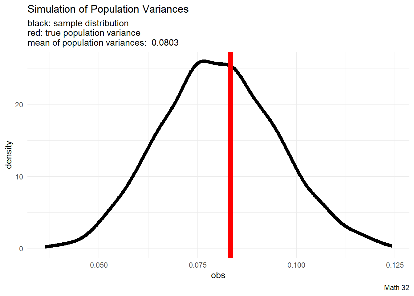

Simulation

Loosely speaking, since the sampling distribution tends to underestimate the population variance, we say that the population variance (with $N$) is a biased estimator of the population variance.

Bessel’s Correction

Can we rescale the process for computing variance so that the operation is an unbiased estimator for the population variance?

Let $X_i$ be a set of $n$ i.i.d. random variables from the same distribution with the same population variance ${\sigma }^2$. By independence, there is zero covariance.

We will compute the value of $k$ so that

$$\text{E}[k\cdot \frac{\sum _{i=1}^n(X_i-{\overline{X}}_n{)}^2}{n}]={\sigma }^2$$

Lemma: $\text{Var}(X_i-{\overline{X}}_n)={\displaystyle \frac{n-1}{n}\cdot {\sigma }^2}$

Bessel’s Correction

We have derived the formula for the sample variance

$$S_n^2={\displaystyle \frac{1}{n-1}{\displaystyle \sum _{i=1}^n(X_i-{\overline{X}}_n{)}^2}}$$

That is, the “$n-1$” (Bessel’s correction) is in place so that the sample variance $s^2$ is an unbiased estimator of the population variance ${\sigma }^2$

Sample Variance

Setup

We will run simulations with $X\sim U(0,1)$ because we know what the answers should be. The population variance is

$${\sigma }^2={\displaystyle \frac{(b-a{)}^2}{12}={\displaystyle \frac{1}{12}}}$$

We will explore what happens if we apply the sample variance formula

$$s^2=\frac{1}{n-1}{\displaystyle \sum _{i=1}^n(x_i-\mu {)}^2}$$

to samples.

Code

# user-defined function
samp_var <- function(x){
  n  <- length(!is.na(x)) #sample size
  xbar <- mean(x, na.rm = TRUE) #sample mean
  
  # return population mean (note use of "n-1")
  sum( (x - xbar)^2 ) / (n-1)
}

N <- 1337 # number of iterations
n <- 25   # sample size

# pre-allocate vector of space for observations
obs <- rep(NA, N)

# run simulation
for(i in 1:N){
  these_numbers <- runif(n, 0, 1) # sample n numbers from U(0,1)
  obs[i] <- samp_var(these_numbers) #record sample variance
}

# mean of observations
mean_of_obs <- mean(obs)

# make data frame
df <- data.frame(obs)

# visualization
df |>
  ggplot(aes(x = obs)) +
  geom_density(color = "black", size = 2) +
  geom_vline(xintercept = 1/12, color = "red", size = 3) +
  labs(title = "Simulation of Sample Variances",
       subtitle = paste("black: sample distribution\nred: true population variance\nmean of sample variances: ", round(mean_of_obs, 4)),
       caption = "Math 32") +
  theme_minimal()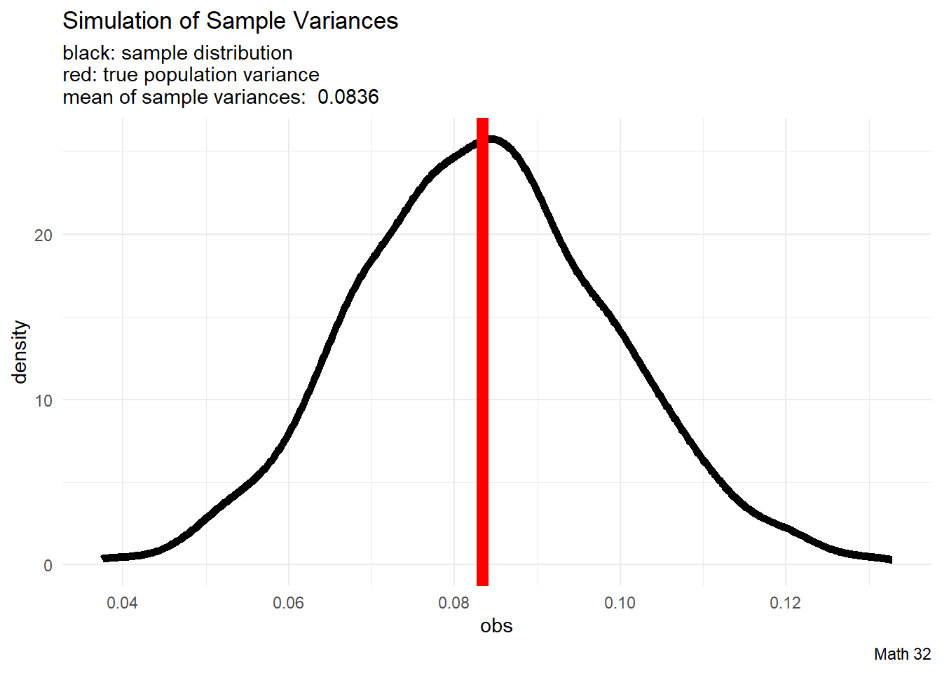

Simulation

Loosely speaking, since the sampling distribution “lines up” with the population variance, we say that the sample variance (with $n-1$) is an unbiased estimator of the population variance.

Sample Standard Deviation

Setup

We will run simulations with $X\sim U(0,1)$ because we know what the answers should be. The population standard deviation is

$$\sigma =\sqrt{{\displaystyle \frac{(b-a{)}^2}{12}}}=\sqrt{{\displaystyle \frac{1}{12}}}$$

We will explore what happens if we apply the sample variance formula

$$s=\sqrt{\frac{1}{n-1}{\displaystyle \sum _{i=1}^n(x_i-\mu {)}^2}}$$

to samples.

Code

# user-defined function
samp_var <- function(x){
  n  <- length(!is.na(x)) #sample size
  xbar <- mean(x, na.rm = TRUE) #sample mean
  
  # return population mean (note use of "n-1")
  sum( (x - xbar)^2 ) / (n-1)
}

N <- 1337 # number of iterations
n <- 25   # sample size

# pre-allocate vector of space for observations
obs <- rep(NA, N)

# run simulation
for(i in 1:N){
  these_numbers <- runif(n, 0, 1) # sample n numbers from U(0,1)
  obs[i] <- sqrt(samp_var(these_numbers)) #record sample standard deviation
}

# mean of observations
mean_of_obs <- mean(obs)

# make data frame
df <- data.frame(obs)

# visualization
df |>
  ggplot(aes(x = obs)) +
  geom_density(color = "black", size = 2) +
  geom_vline(xintercept = sqrt(1/12), color = "red", size = 3) +
  labs(title = "Simulation of Sample Variances",
       subtitle = paste("black: sample distribution\nred: true population variance\nmean of sample standard deviations: ", round(mean_of_obs, 4)),
       caption = "Math 32") +
  theme_minimal()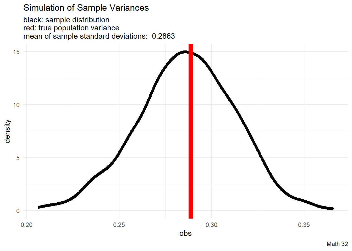

Simulation

Commentary

Let $X_i$ be a set of $n$ i.i.d. random variables from the same distribution with the same population standard deviation $\sigma$. To avoid trivial situations, assume non-zero variance, so $\sigma \ne 0$.

If $s=\sqrt{{\displaystyle \frac{\sum _{i=1}^n(X_i-{\overline{X}}_n{)}^2}{n-1}}}$ was an unbiased estimator, then $\text{E}[s]=\sigma$

However, by Jensen’s Inequality, since $g(x)=x^2$ is a convex function,

$${\sigma }^2=\text{E}[S_n^2]>{(\text{E}[S_n])}^2$$

and it follows that $\text{E}[S_n]<\sigma$. Due to the underestimation, sample standard deviation $s$ is a biased estimator of population standard deviation $\sigma$.

$$$$

However, in practice, the discrepancy is usually so small that it is ignored.

Looking Ahead

• due Fri., Mar. 24:

  • LHW8

• no lecture on Mar. 24, Apr. 3

• Exam 2 will be on Mon., Apr. 10